2026-03-08

Measuring the Pipeline

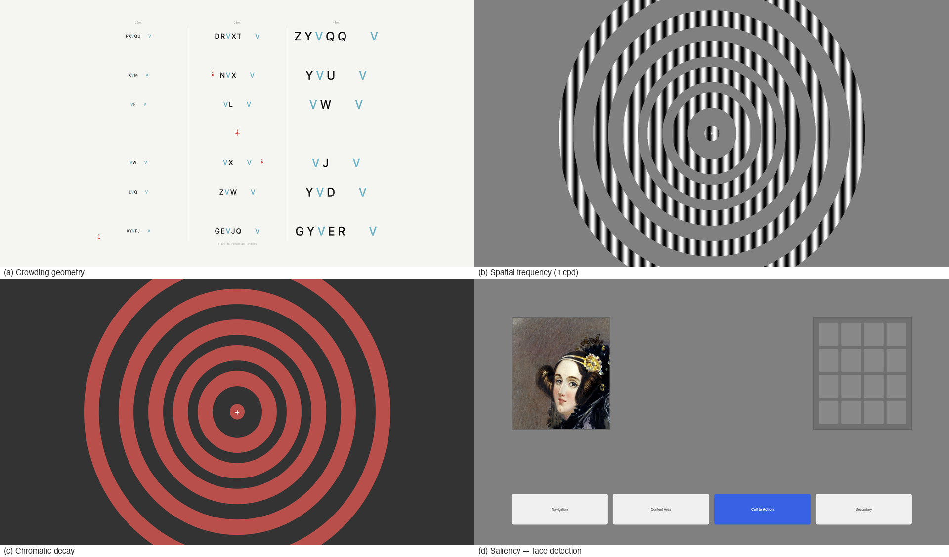
v2.0 made the pipeline visible. v2.1 asks whether it’s correct. We rebuilt five classic human vision experiments as automated reference pages, ran the shader against each one, and compared pixel measurements to the published data. The whole battery — stimulus pages, capture scripts, analysis, golden captures — ran in a single day. Three shader bugs fell out that prior testing had not caught.

• Chromatic decay — Mullen 2002, Hansen 2009, Bowers 2025
• Spatial frequency — Rovamo & Virsu 1979
• Crowding geometry — Bouma 1970, Toet & Levi 1992
• Saliency protection — Itti & Koch 2001, Hershler 2005
• Mixed-density search — Halverson & Hornof 2011

Also in this release: 8 half-octave DoG bands replace the old 4-band decomposition. Smoother blur gradient, twice as many frequency transitions, same API.

Five waves of validation

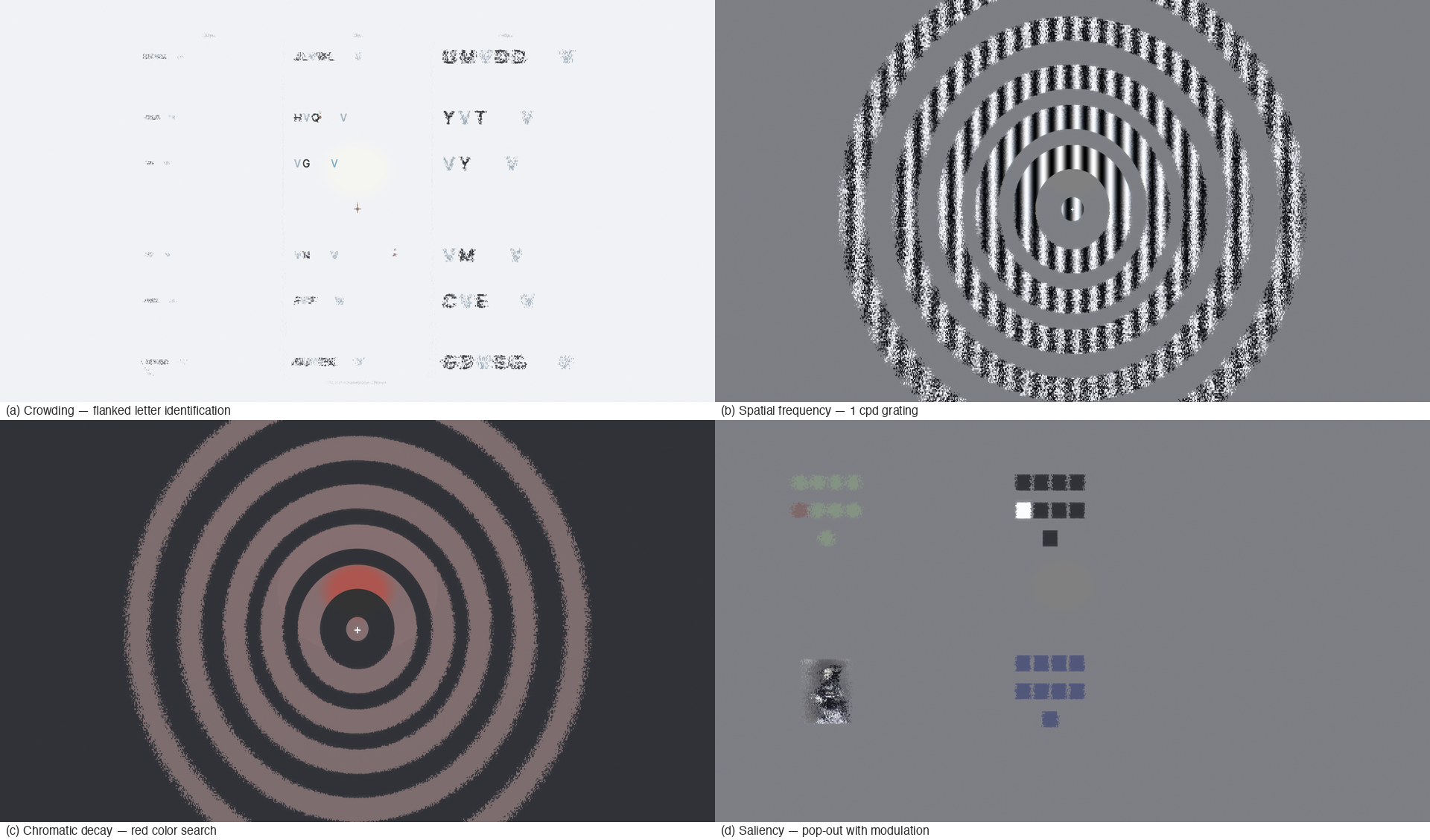
Each wave targets a different stage of the rendering pipeline and emulates a different class of psychophysical experiment. The test pattern is consistent: render a known stimulus through the full shader, measure output pixels, compare against published human data.

The validation infrastructure — 5 capture scripts, 5 analysis scripts, 15 reference pages, 25+ golden captures — now ships with the repository. Every claim in the arxiv paper can be reproduced by running the scripts.

The published data we validated against spans 45 years of vision science, digitized into machine-readable JSON: tests/validation/published-data/

• rovamo_virsu1979_csf.json — contrast sensitivity across 4 spatial frequencies at 7 eccentricities, digitized from Figures 3–6
• hansen2009_color_naming.json — color naming accuracy for 8 hues at 5 eccentricities (0°–50°)
• mullen_kingdom2002_rg_by.json — RG vs BY chromatic sensitivity as a function of eccentricity
• bowers2025_sensitivity.json — suprathreshold chromatic sensitivity from recent eye-tracking measurements

What the validation found wrong

Three bugs surfaced through measurement that visual inspection missed:

• Polar sector R:T ratio (Wave 3) — peripheral.frag computed spoke count from biased ring width, cancelling the intended 2:1 radial elongation. The formula produced ~1:1. Toet & Levi (1992) measured ~2:1. Fixed. (a89ed97, 4509e66)
• V1 far-peripheral growth (Wave 3) — Displacement plateaued beyond the parafovea. Growth factor tuned from 0.5 to 1.5 via capture-analyze loop. (2cda534, 3c9376f)
• Rovamo correlation (Wave 2) — Per-band Spearman correlations failed because each band transitions 100%→0% at a single cutoff. Replaced with composite frequency-weighted metric: $r = 0.600$. (b54eb3f)

Two limits we found

• Stepped blur, not smooth. The blur transitions in discrete steps rather than continuously. Human vision has a smooth falloff; the GPU architecture forces discrete levels. 8 bands are better than 4, but still stepped.
• Crowding strength, not spacing. The density gate controls how much distortion nearby elements cause, but not the critical spacing at which crowding kicks in. Two letters close together and two letters far apart at the same eccentricity get the same treatment. This is an architectural constraint of per-pixel rendering.

8 half-octave DoG bands

The previous version decomposed the image into 4 frequency bands — fine detail, medium detail, coarse structure, layout. The blur transition from sharp to pooled had 4 steps, which meant the parafoveal region (where text goes from readable to unreadable) had only 1–2 active bands at any point. Coarse.

v2.1 doubles the resolution to 8 bands at half-octave spacing. The blur gradient is now twice as smooth, with the biggest improvement in the critical parafoveal zone. The old 4 bands are still in there (bands 1, 3, 5, 7 below) — the new bands interleave between them.

Performance cost is negligible — under 1ms at 1080p.

Wave 5: Halverson mixed-density

The fifth validation wave tests the density gate against behavioral data from a real UI search task. Halverson & Hornof (2011) built an EPIC cognitive architecture model and found that peripheral encoding accuracy depends on local text density: 90% for sparse text (nearest neighbor ≥ 0.15°), 50% for dense text (< 0.15°).

The stimulus page reproduces their mixed-density search task: 6 word groups in a 2×3 grid, sparse and dense conditions at parametric spacing. The analysis script measures per-group SSIM, edge density ratio, and composite availability — testing whether Scrutinizer’s density gate predicts the same pattern that Halverson validated against 24 participants’ eye-tracking data.

Also in this release

• 15 experimental stimuli — HTML reference pages shipping as open-source psychophysical stimuli. Color search, spatial acuity, crowding (4 variants), saliency pop-out, face detection, Halverson mixed-density. Accessible via Go → Reference Pages.
• Arxiv paper updates — Walton 2021 acknowledged, WebGPU tiered roadmap, mongrel Tier 2.5 spec, expanded Open Problems section.
• TEST_LOAD_TIMEOUT — Heavy external pages that never fire did-finish-load now timeout gracefully.
• Appendix baseline captures — Unfiltered stimuli for arxiv paper appendix figures.

What’s next

The validation pipeline is infrastructure. Now that every change can be measured against published data, the path forward is clearer. Next: orientation-dependent blur (horizontal and vertical edges persist further than diagonal ones in real peripheral vision) and smoother color integration across the visual field.

The density gate holds up under measurement but is still an approximation of the real crowding mechanism. Whether GPU rendering can get closer is an open question.

References cited: Bouma 1970 · Bowers, Gegenfurtner & Goettker 2025 · Halverson & Hornof 2011 · Hansen et al. 2009 · Hershler & Hochstein 2005 · Itti & Koch 2001 · Mullen & Kingdom 2002 · Rovamo & Virsu 1979 · Toet & Levi 1992 — Annotated Bibliography · Primer References