Your Brain's Rendering Pipeline, in 2000+ Lines of GLSL⚙
GLSL (OpenGL Shading Language) is a C-like language that runs directly on
the GPU. A fragment shader is a program that executes once per pixel,
in parallel, every frame — making it ideal for real-time image processing. The entire
foveated vision simulation runs as a single fragment shader at 60fps.
You see the world through a pipeline. Light enters the eye, gets filtered, decomposed,
and reassembled — and at each stage, the periphery gets a different deal than the fovea.
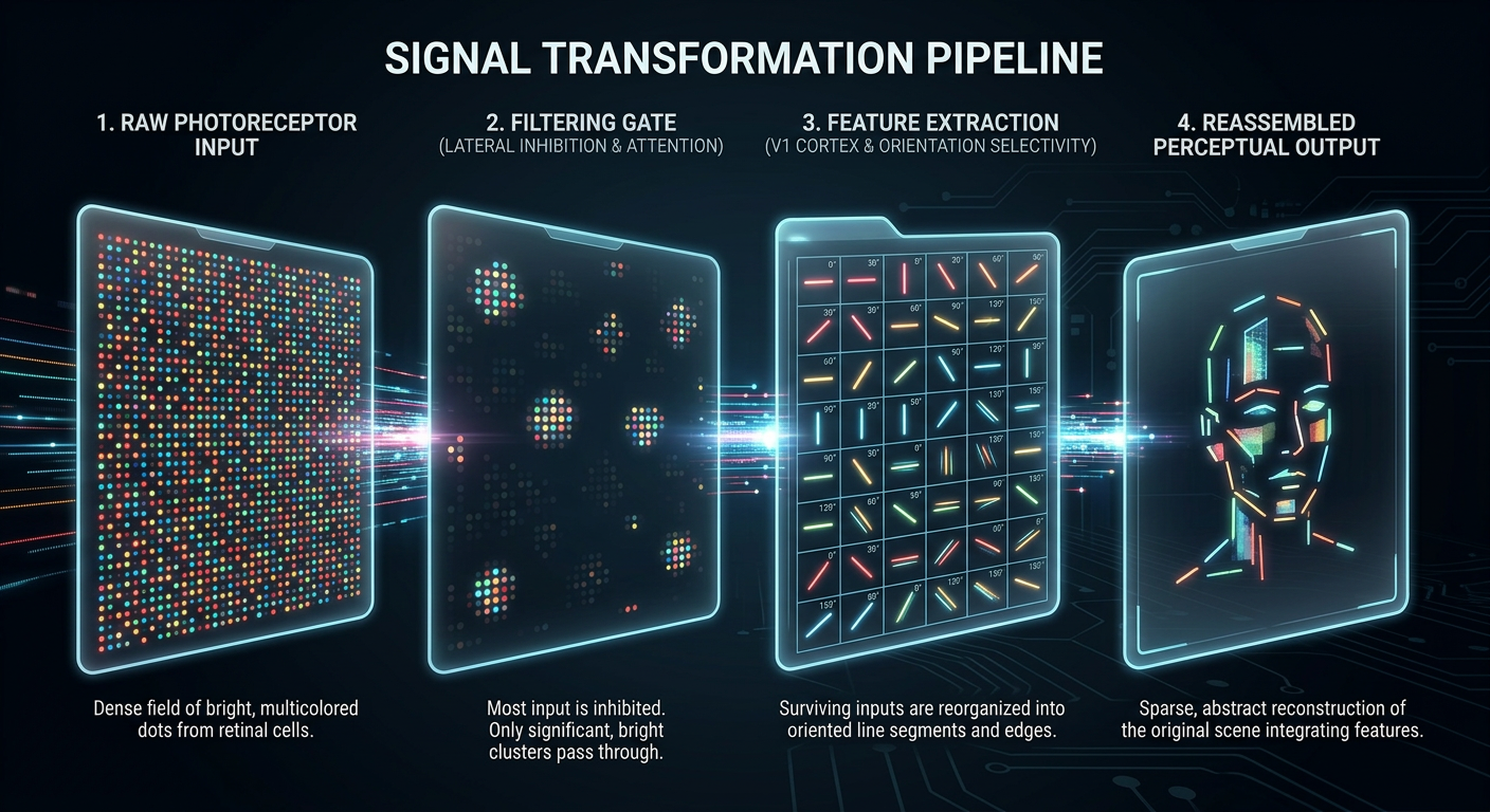
Retina
Photons → electrical signals
LGN
Gates what reaches cortex
V1
Decomposes into features
V4
Color & form processing
What does the signal look like at each stage?
What's preserved, what's lost, and what representation arrives downstream?
Scrutinizer makes those transformations visible. Each biological stage maps to
a real-time shader operation, running on every pixel, every frame.
Retina → LGN → V1 → V4 · implemented in a single GLSL fragment shader
The signal at each stage. Dense photoreceptor input is filtered by the LGN gate,
decomposed into oriented features by V1, and reassembled into a sparse perceptual
representation. Information is progressively refined — not lost, transformed.
The simulation running live on a browser page. Follow the cursor — that's your fovea.
Wrapped in a browser built with the popular Electron framework, the simulation runs on any
web page in real time — turning the screen into a window onto your own visual processing.
The Pipeline: Biology → GLSL
The visual system is vastly more complex than any current simulation captures —
dozens of cortical areas, parallel processing streams, recurrent feedback loops.
The shader models four stages chosen for their outsized impact on peripheral
appearance: retinal spatial filtering, LGN attentional gating, V1 feature integration,
and V4 color processing. Eccentricity from the gaze point drives every parameter.
$\vec{P}_{\text{fragment}}$ is the screen position of the current pixel (in GPU terminology,
a fragment — the shader runs this equation independently for every pixel on screen,
every frame). $\vec{P}_{\text{gaze}}$ is the current gaze point (mouse position or eye-tracker input).
At eccentricity = 0, you're at the fovea (full detail). At 1.0, you're at the foveal boundary.
At 2.5, parafovea. Beyond that: peripheral vision, where most of the visual field lives — and
where most of the shader's work happens.
Biological Primer
The retina is not a passive sensor — it's a layered neural circuit.
The sections below summarize the minimum context for following the simulation.
The key structures — retina, LGN, V1, V4 — have been well characterized since
Kuffler (1953) and Hubel & Wiesel (1962).
Receptive Field Mosaic
Each circle represents one ganglion cell's receptive field.
Dense, small fields at the fovea; sparse, large fields in the periphery. This is
why peripheral vision loses spatial detail: fewer cells, each pooling a wider region.
The Retina: Where Vision Begins
Light hits photoreceptors (rods and cones), which convert photons to
electrical signals. These signals pass through bipolar cells to
retinal ganglion cells, whose axons form the optic nerve.
In the fovea — a 1.5mm pit at the retina's center, densely packed with
cones — each cone connects to its own ganglion cell (1:1 wiring). In the periphery,
100+ rods converge onto a single ganglion cell, trading spatial resolution for sensitivity.
This convergence ratio is the fundamental reason peripheral vision loses detail — signals
are pooled, not lost. You can detect that something is there, but you can't tell what it is.
Photoreceptor Convergence
Photoreceptors (top) funnel onto ganglion cells (bottom).
At the fovea, each cone has its own dedicated ganglion cell (1:1). In the periphery,
dozens of rods converge onto a single cell with a large receptive field —
gaining sensitivity, losing spatial resolution.
Receptive Fields and Center-Surround🔬
Kuffler's 1953 experiment was elegantly simple: he recorded from individual ganglion cells
in the cat retina while shining small spots of light at different positions. He found that
each cell responded to a specific patch of the visual field — its receptive field — and
that a spot in the center excited the cell while a spot in the surround inhibited it (or vice versa).
This center-surround antagonism is the retina's first act of computation: extracting contrast,
not absolute brightness.
A neuron's receptive field is the region of visual space that drives its
response. Retinal ganglion cells have center-surround receptive fields
(Kuffler, 1953): an excitatory center ringed by an inhibitory surround, or vice versa.
The Difference-of-Gaussians (DoG) is a mathematical model of this response profile.
Center-surround organization makes these neurons bandpass filters — they respond
to spatial frequencies matching their field size, not to uniform illumination.
Receptive field size scales with eccentricity: larger fields in the periphery
means coarser frequency tuning further from fixation.
The Visual Pathway
Signals leave the retina via the optic nerve and pass through a series of
processing stages before reaching cortex.
Lateral Geniculate Nucleus (LGN)
A six-layered thalamic relay. Magnocellular layers (fed by
parasol ganglion cells) carry fast, achromatic, motion-sensitive signals.
Parvocellular layers (fed by midget ganglion cells) carry slower,
color-sensitive, high spatial frequency signals.
V1 (primary visual cortex)
Orientation-selective neurons (Hubel & Wiesel, 1962) decompose the image
into local features — edges, bars, gratings at specific angles.
V4
Processes increasingly complex properties: contours, color constancy,
object recognition.
Eccentricity and the Three Zones
0–2°
Fovea — highest acuity, cone-dominated
2–5°
Parafovea — crowding begins
5°+
Periphery — coarse spatial pooling
Eccentricity is the angular distance from fixation, measured in degrees of
visual angle. The cortex devotes disproportionate surface area to the fovea — a property
called cortical magnification (M-scaling). This is why a letter at 10°
eccentricity must be ~5x larger than a foveal letter to be equally legible.
"The LGN is not a relay station. It's a gate."
— Sherman & Guillery, The role of the thalamus in the flow of information to the cortex (2002)
The LGN as Sherman & Guillery describe it — a gate sitting on the signal path,
with a control input wired from cortex. Feed-forward signal flows
retina → LGN → V1 → V4. The dashed gold
arrow is the cortico-thalamic feedback: V1 telling the LGN what
to let through. The post-gate beam is visibly narrower than the pre-gate beam —
not everything the retina captures reaches cortex, and what reaches cortex is
what cortex asked for.
The Lateral Geniculate Nucleus sits between retina and cortex. For decades, neuroscientists
treated it as a simple relay — signals pass through unchanged. Sherman and Guillery showed
it's actually an attentional gatekeeper: top-down signals from cortex modulate what gets
through. If you've built information retrieval systems, this is a familiar pattern —
a filter stage that decides what enters the processing pipeline at all, before any
expensive downstream computation. In the shader, this gating is instantiated as two
binary switches and a multiplication. The signal either passes or it doesn't.
Structure Masking⚙
The structure map is packed into a standard RGB texture — a pragmatic reuse of an
existing GPU data structure. Each pixel encodes three signals as color channels, which
the shader reads as vec3 components. No custom buffer formats or additional
render passes needed — the GPU's texture sampling hardware does the interpolation for free.
The LGN gate needs to know what kind of content occupies each region of the page —
and how that knowledge is represented constrains what operations are natural downstream.
A content analysis pass (content-analysis.js) scans the DOM and encodes
three signals into a structure map:
Rhythm — text cadence and repetition (are there regular line breaks, list items, tabular patterns?)
Density — visual weight per region (dense paragraph vs. whitespace vs. sparse navigation)
Type — element classification (text, image, interactive control, empty)
When the LGN stage encounters low density — empty whitespace between content — it
suppresses the downstream simulation entirely. The biological LGN doesn't gate blank
space to cortex; the simulation mirrors this by zeroing the suppression factor for
regions with no visual content to process.
// LGN Structure Masking — lines 319–323 of peripheral.fragif (config.lgn_use_structure_mask) {
if (u_has_structure > 0.5 && signal.density < 0.1) {
signal.suppressionFactor = 0.0; // Skip peripheral simulation for empty space
}
}
Saliency Gating
The saliency map (edge detection + color contrast, temporally smoothed;
pop-out reference) tells the LGN
what deserves processing bandwidth. This is the same problem biology solves:
the retina captures ~107 bits/sec but the optic nerve transmits ~106.
The visual system doesn't "degrade then un-degrade" — it selectively allocates limited
processing resources to high-value input. Our simulation mirrors this: salient regions
receive reduced peripheral filtering (the simulation's analogue of preferential
processing), while low-saliency regions are processed cheaply.
At saliency=1.0, the suppression factor drops to 0.3 — the pipeline passes most of the
original signal through. At saliency=0.0, full peripheral filtering applies.
Both biology and simulation share the same driver: compute demand management.
foveaparaperiph
Dashboard — center focus. The fovea reveals full detail at
gaze point. Peripheral regions are filtered through the full LGN→V1→V4 pipeline.
Saliency map. Bright = high saliency = more processing bandwidth
allocated. Text blocks, faces, and colored status badges demand the most resources.
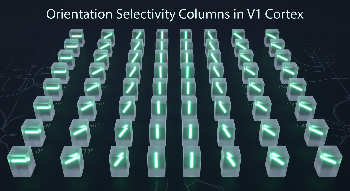
V1 orientation columns. Each cortical column responds to edges at a specific angle —
0°, 30°, 60°, 90°, 120°, 150°. This is how the brain decomposes the visual signal
into oriented features (Hubel & Wiesel, 1962).
After the LGN gate, the signal that survives enters V1 — and here the nature of
the representation changes fundamentally. Primary visual cortex decomposes the
signal into features: orientation, spatial frequency, motion. In the periphery, these features
are extracted at progressively lower resolution — receptive fields grow larger,
features crowd into each other, and positional certainty degrades.
Scrutinizer's V1 stage implements three key peripheral phenomena: positional
uncertainty (domain warping), crowding (feature scrambling),
and spatial pooling (resolution loss). The LGN's suppression factor
modulates all of them — up to 25% attenuation for salient content.
Domain Warping: Positional Uncertainty
In the periphery, you can detect that something is there but not where
exactly it is. Scrutinizer simulates this with fractal noise displacement — two octaves
of Simplex noise at 150x and 300x frequency, with an anisotropic 2x radial bias
(crowding is more severe along the radial axis toward/away from fixation than tangentially;
Toet & Levi 1992).
Where $s$ = distortion strength (eccentricity-scaled) and $I$ = intensity.
The 0.0024 constant maps perceptual data: at the foveal boundary, displacement
is ~2 pixels. At the far periphery, ~24 pixels — a 12x range matching empirical crowding zones.
Crowding: The Fundamental Limit
"Crowding is not blur." — Denis Pelli (2008). You can detect a letter in your periphery.
You cannot identify it when flanked by other letters. The bottleneck isn't resolution —
it's obligatory feature integration across the receptive field.
This is arguably the most important phenomenon in peripheral vision — and it's an
information-theoretic one (crowding reference stimuli,
Bouma spacing).
Crowding determines not what you can't see, but what
you can't separate. Adjacent features are compulsorily pooled — averaged,
texture-ified — once they share a receptive field. The information isn't gone; it's been
irreversibly mixed. The individual signals are still in there, but the representation
can no longer distinguish them. Bouma's law quantifies the critical spacing:
Bouma's Law — Critical Spacing
$$s \approx 0.5 \cdot \phi$$
Where $s$ = minimum spacing to avoid crowding and $\phi$ = eccentricity from fixation.
At 10° eccentricity, targets must be ≥5° apart to be individually identified.
This linear scaling with eccentricity mirrors cortical magnification — it's the same
constraint expressed differently.
The shader implements two crowding modes:
Fractal Noise — Continuous warp via Simplex noise, increasing amplitude with eccentricity. Preserves overall structure but scrambles local features.
Discrete Scramble — Grid-based cell shredding. Each cell gets a random displacement vector, creating a "shattered glass" effect. Saliency guides where the grid breaks.
Article — center focus. V1 crowding filters paragraph text in the periphery
while headlines receive more bandwidth (larger receptive fields).
foveaparaperiph
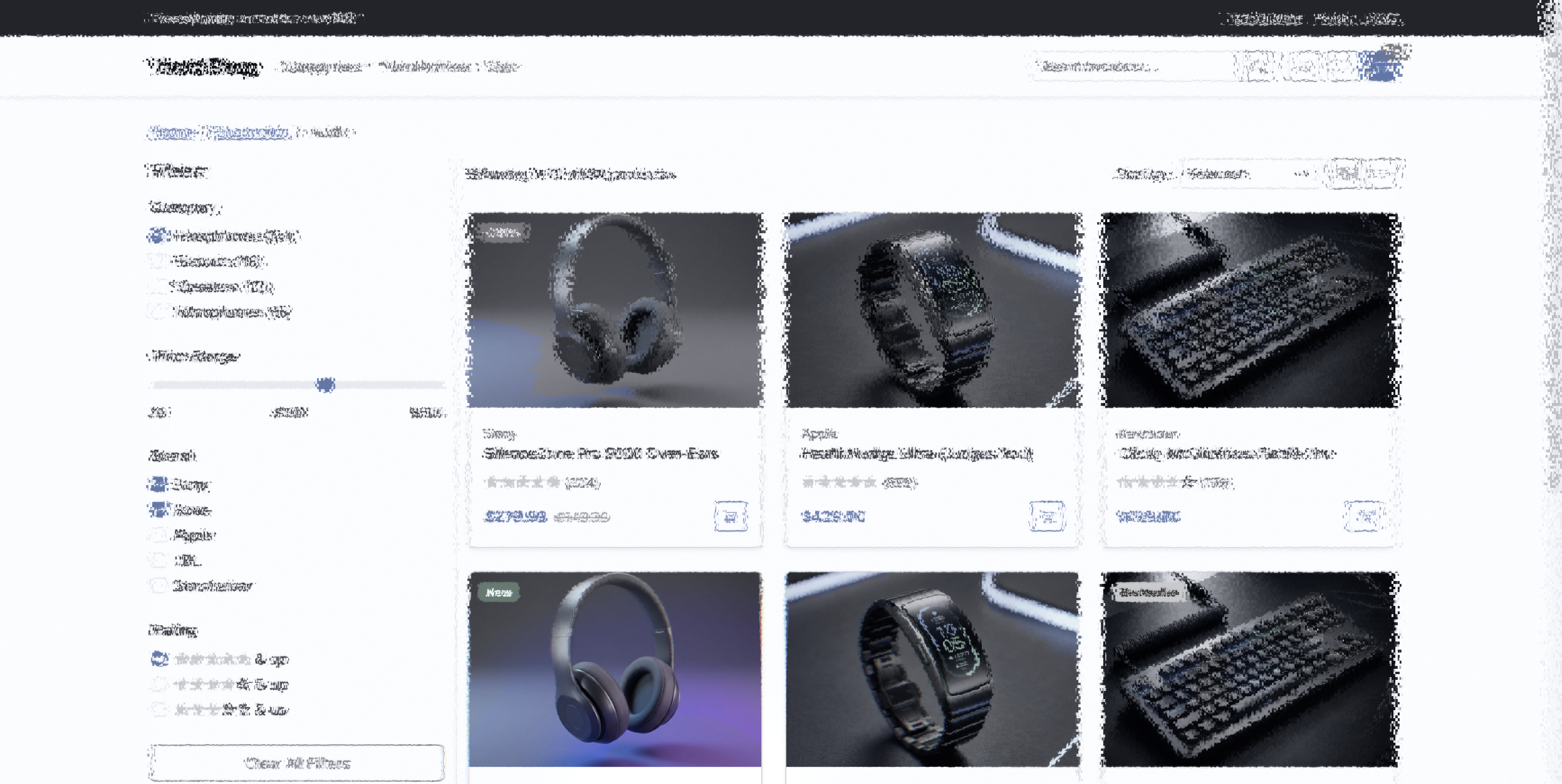
E-commerce — product focus. When you fixate on the product image,
the price tag, CTA button, and reviews are filtered through V1 scrambling — a visualization
of the feature pooling that constrains peripheral object recognition.
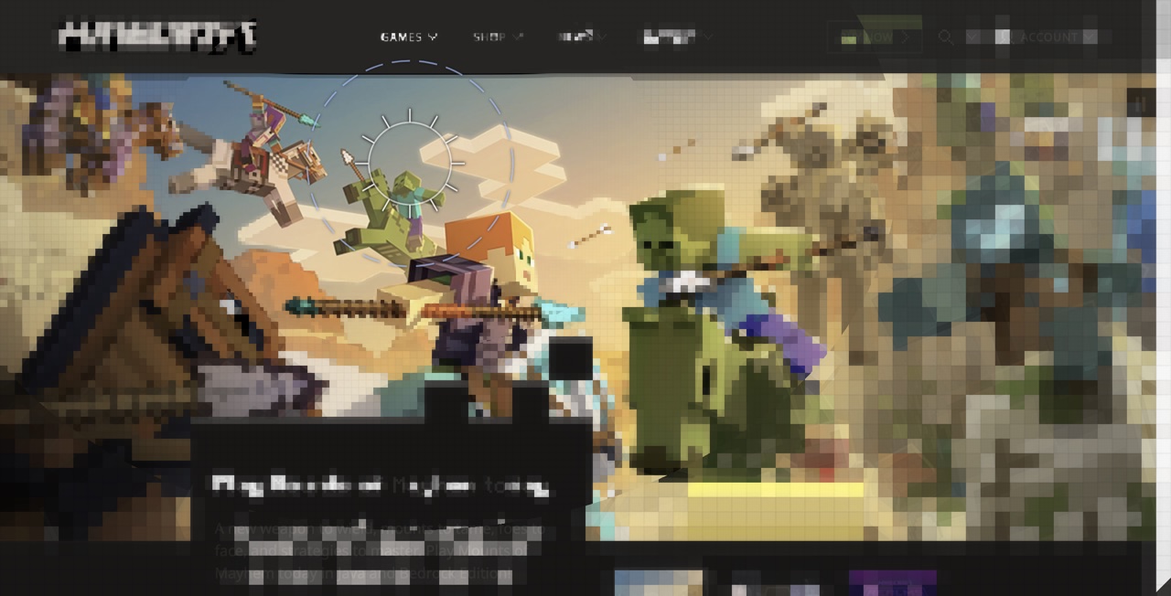
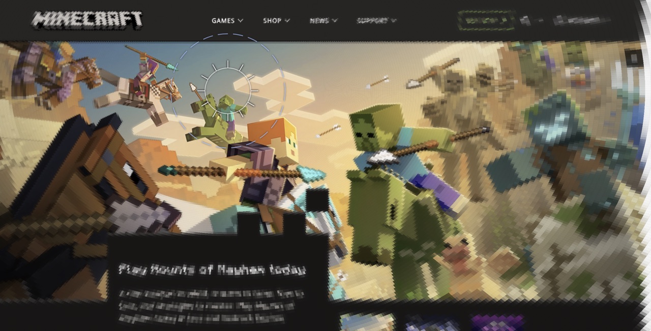
Two presentation modes make the pooling geometry tangible. Minecraft quantizes
the image into blocks sized by cortical magnification — 4px at the fovea, 64px in the far
periphery. Each block shows the mean color of its receptive field. MC Eyeball
does the same with polar sectors radiating from the gaze point, matching the radial elongation
of TTM pooling regions (Toet & Levi 1992).
Minecraft (Block Pooling). Blocks grow with eccentricity,
showing the cortical magnification function as visible geometry. Fine blocks at the fovea,
coarse blocks in the periphery.
MC Eyeball (Polar Pooling). Wedge-shaped sectors
emanate from the gaze point, radially elongated ~2:1. This is what TTM pooling regions
look like — the geometry the summary statistics are computed within.
Toward Mongrel Textures: DoG Band Decomposition
By the time the signal reaches the periphery, what does the representation actually
contain? Rosenholtz et al. (2012) answered this precisely:
summary statistics — local texture-like representations that
preserve aggregate properties (mean color, dominant orientation, spatial frequency
distribution) while discarding individual feature identity.
A lossy compression where the encoder is the visual system itself.
Rosenholtz's mongrel images, synthesized to match these statistics, are
perceptually indistinguishable from the original in the periphery. The catch:
synthesizing mongrels takes ~30 minutes per image on current hardware (M3 MacBook
with MPS acceleration, 300 optimization iterations).
Real-Time Approximation
The shader's DoG band decomposition approximates this at real-time rates. Rather than
computing full texture statistics, it decomposes the image into spatial frequency bands
and attenuates them independently based on eccentricity. Fine detail drops out before
coarse structure — matching the biological attenuation profile where retinal ganglion
cells act as bandpass filters whose size scales with eccentricity
(Curcio et al., 1990).
The Approximate Laplacian Pyramid⚙
A MIP chain (from Latin multum in parvo, "much in little") is a
series of progressively downsampled copies of a texture that GPUs generate automatically.
Level 0 is the full-resolution image; level 1 is half-resolution; level 2 is quarter, etc.
GPUs use these for texture filtering at different distances. Hardware MIP generation uses
box or bilinear filtering — not the Gaussian convolution of a true Laplacian pyramid
(Burt & Adelson, 1983). The shader repurposes this existing hardware feature:
subtracting adjacent MIP levels produces an
approximate Laplacian pyramid, where each level captures a band of spatial
frequencies with some spectral leakage between bands.
The shader decomposes the hardware MIP chain into an approximate Laplacian pyramid —
each band captures a spatial frequency range:
Band 01–2 px: serifs, thin strokes
Band 12–4 px: letter bodies, small icons
Band 24–8 px: words, UI elements
Band 38–16 px: buttons, layout blocks
ResidualDC: overall color & luminance (always preserved)
Each band has its own cutoff eccentricity — the distance from the fovea where that
frequency band is fully attenuated. With 8 half-octave bands, the cutoffs follow
$\sqrt{2}$ spacing, matching the $E_2$ scaling of cortical magnification
(validated against published contrast sensitivity data —
see report):
Where $E_2$ is the half-resolution eccentricity — the point where spatial resolution
drops to half its foveal value. In the shader: u_dog_e2, user-adjustable.
Odd-indexed cutoffs ($c_1, c_3, c_5, c_7$) match the original 4-band anchor values.
Each band's weight is computed via smoothstep rolloff, with a transition width controlled
by u_dog_sharpness. At sharpness=0, the transitions are wide and gradual
(biological). At sharpness=1, they're narrow and crisp (engineering utility mode).
// Per-band weights via smoothstep rollofffloat w[8];
for (int k = 0; k < 8; k++) {
w[k] = 1.0 - smoothstep(c[k] - c[k]*trans, c[k] + c[k]*trans, normEcc);
}
// Reconstruction: residual + weighted bands
result = mip[8];
for (int k = 0; k < 8; k++) { result += band[k] * w[k]; }
result = clamp(result, 0.0, 1.0);
What This Means in Practice
Fine detail filters first, coarse structure passes through longest. The signal isn't
uniformly blurred — it's selectively attenuated by frequency band.
Close to the fovea, all 8 bands survive — full detail. In the parafovea, the finest bands
(serifs, thin strokes) drop out first. You can still read words but individual letterforms
lose their character. Further out, letter-body bands fade — shapes become blobs. In the far
periphery, only the coarsest bands and the DC residual remain: you see buttons and layout
blocks but not their labels.
Structure map — article. The content analysis feeds the LGN.
Red channel = text rhythm, Green = density, Blue = element type. DoG band weights
are modulated by this structure.
foveaparaperiph
Techmeme — center focus. Dense news layout. DoG preserves
headline structure while filtering individual link text. The data table density is exactly
the kind of content where DoG outperforms uniform blur.
Fidelity Gap: What DoG Misses
The DoG decomposition captures frequency-selective attenuation but not the full
mongrel texture model. True summary statistics include orientation distributions,
phase correlations, and cross-scale feature conjunctions that our isotropic bands
discard. Adding oriented DoG filters — even just horizontal/vertical — would
double the texture lookups but could capture the anisotropy of real V1 receptive
fields (Gabor-like, phase-sensitive). The gap between our real-time approximation
and a full Rosenholtz-style synthesis is where future work lives.
Visual area V4 processes color, shape, and object recognition. In the periphery,
color perception shifts dramatically — the transition from cone-dominated (foveal) to
rod-dominated (peripheral) processing alters hue sensitivity, saturation, and spectral
response (per-channel chromatic decay validated —
see report). The shader's V4 stage simulates these shifts using Oklab color space,
rod-spectrum tinting, and selectable aesthetic rendering modes.
Oklab: Perceptually Uniform Desaturation⚙
A color space is a coordinate system for describing colors. RGB maps
to hardware (red/green/blue light intensities) but doesn't correspond to human perception —
equal RGB steps don't look like equal brightness steps. Perceptually uniform
spaces like Oklab are designed so that equal mathematical distances correspond to equal
perceived color differences. This matters when you need to smoothly remove color: in RGB,
desaturation causes unwanted hue shifts. In Oklab, you can zero out the chrominance
channels (a, b) and get clean, hue-stable grayscale.
A critical design choice. If you desaturate in RGB or HSL, hue shifts as saturation
drops — warm colors skew yellow, cool colors skew cyan. Oklab (Ottosson, 2020)
separates lightness (L) from chrominance (a, b) in a perceptually uniform space.
Killing a and b channels produces clean grayscale without hue contamination.
Oklab separates lightness from chrominance. Each channel maps to a retinal pathway with
different eccentricity falloff. The shader kills red-green (a) before blue-yellow (b),
matching L/M cone ratio collapse in the periphery.
🌈
$$L_{ab} \cdot \begin{pmatrix} 1 \\ 1 - f \\ 1 - f \end{pmatrix} \quad \text{where } f = \text{smoothstep}(r_{\text{fovea}}, \, r_{\text{fovea}} \cdot k, \, d)$$
$f$ = desaturation factor, ramping from 0 at the foveal edge to 1 at the ramp end.
Lightness is preserved. Only chrominance fades. The red-green axis (Oklab a)
is suppressed before blue-yellow (b), matching the faster decay of
L−M midget cell opponency with eccentricity (Mullen & Kingdom 2002).
Chromatic Pooling: Why Blue Outlasts Red
The Oklab desaturation above treats both chrominance channels equally. But biology doesn't.
Your visual system has two independent color pathways with very different eccentricity profiles:
Red-Green (L−M) — a foveal specialization. Sharp at the center, degrades fast.
At 15° eccentricity, sensitivity has dropped 71%.
Blue-Yellow (S−(L+M)) — retina-wide. Works almost everywhere.
At 15°, only 21% lost (Bowers, Gegenfurtner & Goettker 2025).
The shader models this asymmetry with independent decay rates per channel.
The practical consequence for web design:
Element
At 5°
At 10°
At 15°
Large blue background
Full color
Full color
~90%
Small red badge (12px)
Uncertain
Low
Gone
Green success icon
Moderate
Low
Gone
Yellow warning banner
Full color
Full color
~85%
Blue and yellow signals persist in the periphery. Red and green degrade early for small elements.
Always provide a luminance difference alongside color — the achromatic channel carries the signal
regardless of chromatic decay.
The visual system processes information through parallel streams from the retina onward.
Parasol ganglion cells (large, fast) feed the magnocellular (M) layers
of the LGN (layers 1–2), carrying luminance contrast and motion signals. Midget ganglion
cells (small, slower) feed the parvocellular (P) layers (layers 3–6),
carrying color and fine spatial detail. These streams remain largely segregated through V1 and into
higher cortical areas — the M-stream drives motion perception (dorsal/where pathway), while the
P-stream drives object recognition (ventral/what pathway). Livingstone & Hubel (1988) established
this segregation; it explains why you can detect motion in far peripheral vision where color and
form have long since degraded.
The magnocellular (M) pathway — fast, achromatic, motion-sensitive — preserves luminance
contrast even as the parvocellular (P) pathway loses color and detail. The shader samples
the clean (undistorted) image, computes a luminance ratio, and blends it back into the
simulated output. This is why you can still detect edges and motion in your far periphery
even when you can't see color or detail.
Structure map — Techmeme. The structure analysis
that feeds the LGN gate. Dense news sites reveal the rhythm/density/type decomposition
that drives the entire pipeline.
Saliency map — Techmeme. Edge detection + color contrast in Oklab space.
Bright regions receive more processing bandwidth through the LGN gate.
Project Trajectory —
374 commits in 98 days, three shader reverts in 30 minutes, and the gap between
biological accuracy and perceptual plausibility. Read the development arc →
Before & after. Original page (left) vs the full LGN→V1→V4 pipeline (right).
The foveal region preserves full detail; the periphery is filtered through every stage described above.
What the Pipeline Models
Each stage of the rendering pipeline corresponds to a biological mechanism in the early visual system.
For implementation details and full citations, see the
scientific literature review.
Biology
What You See
Key Reference
Foveal cone density
Sharp, full-resolution center where you're looking
Curcio et al. 1990
Rod convergence (100:1)
Progressive blur with distance from fixation — spatial frequencies drop out in bands
Rodieck 1965
Ganglion cell receptive fields
Detail loss follows center-surround (DoG) structure, not Gaussian smear
Kuffler 1953
Cortical magnification
Rate of blur increase matches cortical area devoted to each eccentricity
Schwartz 1977; Blauch et al. 2026
LGN attentional gating
Salient regions (faces, text, high-contrast) stay clearer longer
McAlonan et al. 2008
V1 crowding
Peripheral letters jumble and swap — you see them but can't read them
Pelli 2008; Pelli & Tillman 2008
Positional uncertainty
Objects in periphery shift position slightly, worse horizontally
Levi & Klein 1996
Purkinje shift
Reds fade to gray in the periphery while blues persist
Mullen 1991
Rod spectral sensitivity
Far periphery takes on a cool, slightly cyan cast
Wald 1945
Magnocellular pathway
Contrast and motion structure preserved even when color and detail are gone
Merigan & Maunsell 1993
Saccadic suppression
Brief blur during rapid eye movements — you don't notice your own saccades
Burr et al. 1994
Eigengrau
Dark regions never go fully black — the visual system has a baseline "gray"
Barlow 1957
Mobile: The Smaller Fovea
On mobile, the fovea subtends the same visual angle, but the screen is held closer and
the viewport is denser. The simulation reveals something counterintuitive: much of the content
on a phone screen sits in the parafoveal zone — not the far periphery, but the transitional
region where feature integration begins to degrade. This is where crowding first bites.
foveaparaperiph
iPhone 14 — article. The same article page at mobile scale.
Much of the content sits in the parafoveal zone, where feature integration starts to pool individual elements into texture.
foveaparaperiph
iPhone 14 — dashboard. Data-dense UIs on mobile. The fovea
reveals one card; most content falls into parafoveal territory.
foveaparaperiph
iPad Air — article. Tablet's larger viewport provides a middle ground. More foveal real estate, but still significant parafoveal load.
foveaparaperiph
iPad Air — dashboard. The data table density makes
this an ideal test case for the DoG band decomposition — rows fade by spatial frequency,
not uniformly.
Andy Edmonds studied cognitive science at Carnegie Mellon, Georgia Tech, and Clemson,
then left academia in 1995 for what became two decades of machine learning at scale —
shipping recommendation systems, search relevance, and information retrieval products at
eBay, Adobe, Microsoft, and Meta.
CMU · Georgia Tech · Clemson|eBay · Adobe · Microsoft · Meta
The through-line: how does information flow through a system, and what happens
to the signal at each stage? Scrutinizer applies that question to the visual system.
The retina decomposes. The LGN gates. V1 pools. V4 recolors — each stage mapping
cleanly onto GPU operations.